����ý

Manufacturing dashboards offer a real-time snapshot of the state of your production processes. The goal is to provide decision-makers with a fast, easy way to access KPIs and other important insights.

Crucially, this replaces the need to manually crunch numbers each time you need the figures in question.

Any time we set out to build dashboards, the biggest challenge is getting all of the different data that we need into one location, formatted compatibly.

Today, we’re checking out how ����ý makes it easier than ever to output professional dashboards based on existing data sources.

But, before we get to that, let’s get to grips with the basics.

What is a manufacturing dashboard

A dashboard is a reporting UI that connects to an external data source. That way, users can view the most up-to-date figures for whatever information we’ve configured our dashboard to display, each time they access it.

The goal is to simultaneously reduce admin workloads and improve access to key information.

In the specific case of a manufacturing dashboard, this will typically concern data relating to our productivity, efficiency, incidents, breakages, costs, or other KPIs.

As such, we might need to draw on a fairly diverse data set - comprising our manufacturing output, incident reports, machinery, and more.

With that in mind…

What are we building?

Today, we’re going to be building a relatively simple, single-screen manufacturing dashboard.

This is going to focus on the current month’s productivity, quality control, breakages, and incidents - across two manufacturing sites - breaking various KPIs down by machine, location, and product.

Here’s what we’ll have by the end:

To achieve this, we’re going to connect to our manufacturing database, which is stored in an external PostgreSQL instance.

This is made up of five interrelated tables, called production, machines, qa, breakages, and incidents.

We’re going to create custom queries within ����ý to extract the information we need from these - and then use this to populate our display elements. ����ý is the ideal solution for SQL pros who need to turn data into professional UIs.

You might also like our guide to open-source low-code platforms .

Let’s dive right in.

How to build a manufacturing dashboard in 5 steps

If you haven’t already, sign up for a free ����ý account.

1. Create a ����ý app and connect your data

The first thing we need to do is create a new ����ý application. We can use a template or import an existing app file, but we’re starting from scratch. We then need to give our app a name and URL extension:

Then, we’re asked which data source we’d like to connect to first:

����ý offers dedicated connectors for a huge range of SQL and NoSQL databases, alongside REST, Google Sheets, and our internal database.

As we say though, we’re using Postgres today.

When we select this, we’ll be prompted to enter our configuration details:

We can then choose which of the constituent tables we want to fetch so that we can manipulate them in ����ý:

Straight away, we can use ����ý’s back-end to perform CRUD actions on our tables or alter their schemas, without writing a single query:

But, we’re primarily going to rely on custom queries to transform and aggregate our data in order to build a manufacturing dashboard.

So, let’s quickly get to grips with what’s stored in our tables and how they all relate to each other:

• production represents the product that we create, with a unique id and product, date, and turnaround_time_minutes attributes. This also stores a machine_id which corresponds to the id attribute in the machines table.
• machines store a unique id, location, and machine_name. The possible locations are Texas and Anaheim.
• qa has a unique id and a production_id attribute that relates to the id of the production table. It also stores a description and an attribute called pass_fail which can either be set to Pass or Fail.
• breakages has a unique id, date, and description, as well as a production_id which links it to the production table.
• incidents has a unique id, date, category, and description. It relates to the machines table via an attribute called machine_id.

We’re going to write several custom queries that aggregate and transform data points from different combinations of these tables to build our various UI elements.

2. Building our summary cards

The first thing we‘re going to do is head to the design section and create a new blank screen. We can call this anything we like, as our dashboard is only going to have one screen anyway. We’ve simply set our URL path to “/”.

On this, we’ll first add a headline component.

We’ll open up the bindings drawer to set the text attribute. We can do this with either handlebars or Javascript:

We want our headline to read This Month: followed by the current month in the format “M��/�۳۳۳�”.

To achieve this, we’re going to use the following handlebars expression:

1This Month: {{ date now "MM" }}/{{ date now "YYYY"}}

Beneath this, we’re going to add a container and set its direction to horizontal:

Inside of this, we’ll nest a cards block. This is a preconfigured set of components that we can point at a data source. It will then iterate over this, displaying whichever values we specify for each entry.

When we’re finished, we’ll have three separate cards blocks, each displaying a single card.

The first one will display the current month’s overall pass rate from our qa table.

To calculate this, we’ll create a custom query under our Postgres data source:

We’ll call this one QaPassRateByMonth.

We need the pass_fail and production_id attributes from the qa table and the date and product_name from the corresponding production row.

We want to SELECT the numerical month and year from the date attribute and the COUNT of qa rows where pass_fail is set to Pass. We’ll then divide this by the overall COUNT and multiply by 100.

We’ll use a LEFT JOIN statement between p.id and qa.production_id and GROUP BY year and month.

So, our query is:

 1SELECT
 2
 3 EXTRACT(YEAR FROM p.date)::INTEGER AS year,
 4
 5 EXTRACT(MONTH FROM p.date)::INTEGER AS month,
 6
 7 COUNT(qa.id) FILTER (WHERE qa.pass_fail = 'Pass') * 100.0 / COUNT(qa.id)::FLOAT AS pass_percentage
 8
 9FROM production p
10
11LEFT JOIN qa ON p.id = qa.production_id
12
13GROUP BY year, month
14
15ORDER BY year, month;

The data object this returns looks like:

1{
2
3 "year": 2023,
4
5 "month": 9,
6
7 "pass_percentage": 90
8
9}

Now, head back to the design section, and we’ll point the data field for our cards block to our new query:

Now, it’s displaying three cards - because our sample data goes back three months. In a second, we’ll set a couple of filters so that this only displays the current month.

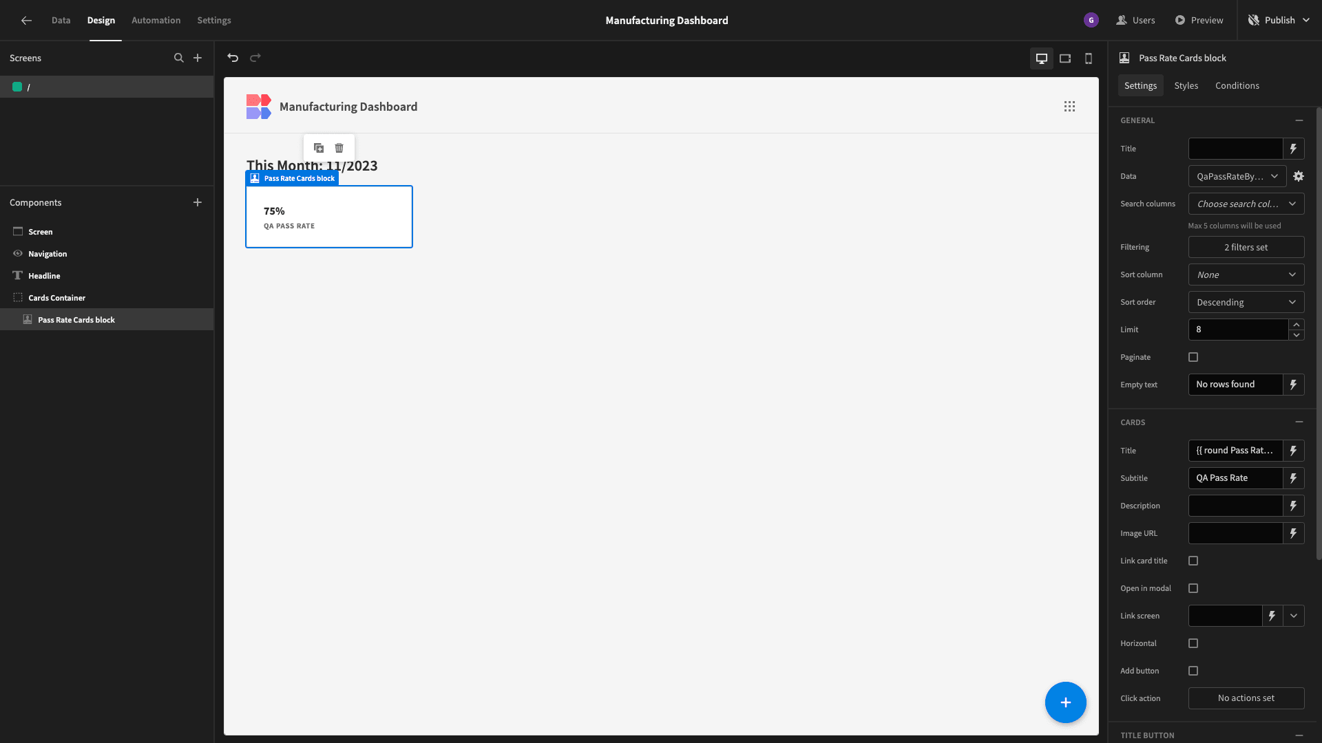
First, though, we want to set the actual data that our cards display.

We’ll start by binding the title to {{ round Pass Rate Cards block.QaPassRateByMonth.pass_percentage }}%.

We’ll also give it a descriptive subtitle and remove the description entirely:

Finally, we’ll add two filtering statements - based on the month and year attributes in our query response:

This time, we’re going to use JavaScript for our bindings instead of handlebars. So, we’ll filter the year against:

1var currentDate = new Date();
2
3return currentDate.getFullYear():

For the month, we’ll use:

1var currentDate = new Date();
2
3return currentDate.getMonth() + 1;

We have to add one here because JavaScript uses zero-based counting for dates. So, the index for January is 0.

Here’s what our filtered cards block looks like:

We’re going to use the same filtering expressions for our other two cards. Rather than configure these from scratch, we’ll make two duplicates of this existing one:

All we need to do is swap out the data.

The second card will show the total number of stock breakages we’ve had this week.

We’ll create a new query called BreakagesByMonth. This time we want to SELECT to COUNT of rows and the numerical month and year from the breakages table, grouped and ordered by month and year.

 1SELECT
 2
 3 EXTRACT(YEAR FROM date)::INTEGER AS year,
 4
 5 EXTRACT(MONTH FROM date)::INTEGER AS month,
 6
 7 COUNT(*)::INTEGER AS breakages_count
 8
 9FROM breakages
10
11GROUP BY year, month
12
13ORDER BY year, month;

The response schema is:

1{
2
3 "year": 2023,
4
5 "month": 9,
6
7 "breakages_count": 5
8
9}

We’ll also create a query called IncidentsByMonth to retrieve the same information from the incidents table.

 1SELECT
 2
 3 EXTRACT(YEAR FROM date)::INTEGER AS year,
 4
 5 EXTRACT(MONTH FROM date)::INTEGER AS month,
 6
 7 COUNT(*)::INTEGER AS incidents_count
 8
 9FROM incidents
10
11GROUP BY year, month
12
13ORDER BY year, month;

This returns:

1{
2
3 "year": 2023,
4
5 "month": 9,
6
7 "incidents_count": 41
8
9}

Now, we can simply swap the data for our new cards to these queries and update the title bindings and subtitles.

Here’s our completed row of cards:

3. Productivity breakdowns

Next, we’ll start building some charts. Add another horizontal container, this time giving it a top margin of 16px:

By the time we’re finished, we’ll have two bar charts inside this, displaying the number of products we’ve created this month - respectively broken down by machine and location.

Start by adding a chart block. This is a preconfigured set of components that accepts a data source and visualizes whichever attributes we tell it to.

We’ll create a new query called ProductionCountByMachineByMonth.

We’ll SELECT the machine_name from machines along with the following from production:

• The numerical month and year.
• The COUNT of the machine_id attribute.

We’ll then LEFT JOIN on m.id = p.machine_id and GROUP BY machine_name, month, and year.

 1SELECT
 2
 3 m.machine_name,
 4
 5 EXTRACT(YEAR FROM p.date)::INTEGER AS year,
 6
 7 EXTRACT(MONTH FROM p.date)::INTEGER AS month,
 8
 9 COUNT(p.machine_id)::INTEGER AS production_count
10
11FROM machines m
12
13LEFT JOIN production p ON m.id = p.machine_id
14
15GROUP BY m.machine_name, year, month
16
17ORDER BY m.machine_name, year, month;

This returns:

 1{
 2
 3 "machine_name": "Machine 1",
 4
 5 "year": 2023,
 6
 7 "month": 9,
 8
 9 "production_count": 7
10
11}

We’ll set the data for our chart block to this query - and choose bar for its type. We’ll also give it a descriptive title:

We also need to configure which attributes will be used for each axis on our graph. We’ll set the label column to machine_name and the data column to production_count:

Just like with the cards, a chart block iterates over the data source we point it at, and displays values for all of the entires. So, we’ll apply the same filters as we did earlier to our month and year attributes in the query response:

Lastly, we’ll add some custom CSS to set the width to 50%:

Here’s our finished chart:

Again, we’ll duplicate this to save ourselves a bit of time:

For the second chart, we’ll use a similar query that calculates the count of products per month, but grouped by the location attribute from the machines table, rather than machine_name.

We’ll call this ProductionCountByLocationByMonth:

 1SELECT
 2
 3 m.location,
 4
 5 EXTRACT(YEAR FROM p.date)::INTEGER AS year,
 6
 7 EXTRACT(MONTH FROM p.date)::INTEGER AS month,
 8
 9 COUNT(p.machine_id)::INTEGER AS production_count
10
11FROM machines m
12
13LEFT JOIN production p ON m.id = p.machine_id
14
15GROUP BY m.location, year, month
16
17ORDER BY m.location, year, month;

This returns:

 1{
 2
 3 "location": "Anaheim",
 4
 5 "year": 2023,
 6
 7 "month": 9,
 8
 9 "production_count": 16
10
11}

Back on the design section, we can swap the data for our second chart to this query’s response:

We’ll also check the horizontal option:

Here’s what we have so far:

4. Breakages and incidents breakdowns

Next, we’ll create our second row of charts. We want a pie chart to show the number of breakages by product and a bar chart showing the incidents by machine.

We’ll start by duplicating our entire existing chart container:

Just like before, we simply need to create new queries to extract the data we want to display, and then swap this out on each of our charts.

We’ll call the first one BreakagesByMonthByProduct. This will SELECT the same information as our original BreakagesByMonth query - but this time also retrieving the relevant product attribute from the production table.

We’ll JOIN breakages to production on b.production_id = p.id.

 1SELECT
 2
 3 EXTRACT(YEAR FROM b.date)::INTEGER AS year,
 4
 5 EXTRACT(MONTH FROM b.date)::INTEGER AS month,
 6
 7 p.product,
 8
 9 COUNT(*)::INTEGER AS breakages_count
10
11FROM breakages b
12
13JOIN production p ON b.production_id = p.id
14
15GROUP BY year, month, p.product
16
17ORDER BY year, month, p.product;

This will return:

 1{
 2
 3 "year": 2023,
 4
 5 "month": 9,
 6
 7 "product": "Ground Screw",
 8
 9 "breakages_count": 1
10
11}

Back on the design screen, we’ll update our third chart to point it at this new query. We’ll also set its type to pie, label column to product, and data column to breakages_count.

Our last query will be called IncidentsByMachine. We need the machine_name from machines, along with the numerical month, year, and COUNT of rows from the incidents table.

We’ll JOIN these on i.machine_id = m.id.

 1SELECT
 2
 3 m.machine_name,
 4
 5 EXTRACT(YEAR FROM i.date)::INTEGER AS year,
 6
 7 EXTRACT(MONTH FROM i.date)::INTEGER AS month,
 8
 9 COUNT(*)::INTEGER AS incidents_count
10
11FROM incidents i
12
13JOIN machines m ON i.machine_id = m.id
14
15GROUP BY m.machine_name, year, month
16
17ORDER BY m.machine_name, year, month;

This will return:

 1{
 2
 3 "machine_name": "Machine 1",
 4
 5 "year": 2023,
 6
 7 "month": 9,
 8
 9 "incidents_count": 12
10
11}

We’ll swap the data for our final chart to match this query response - this time deselecting the horizontal option.

Here’s our manufacturing dashboard so far:

5. Design tweaks and publishing

Before we push this live, we’re going to make a couple of minor UX changes.

First of all, we’ll choose the lightest theme under screen:

Finally, we’ll adjust the color palettes of our charts, to improve visual separation:

Once we’re satisfied, we can publish our app to push it live:

Here’s a reminder of what our finished manufacturing dashboard looks like:

If you found this guide helpful, you might also like our tutorial on how to build an inventory calculator .